maths for quantum computing: quantum circuits.

the story: a little bit of context before the mathematics (feel free to skip)

for some reason i never liked to draw electric circuits in school. my brain sometimes just decides it doesn't like something and i do whatever it takes to avoid it at all costs. when i saw these diagrams i got flashbacks. i thought i could leave this bit behind when it was introduces in week 6, but it's week 11 now and quantum circuit diagrams are here to stay.

in this blog post i aim to compute the final output of a quantum circuit, breaking down the calculation into itty bitty steps and annotating the diagram. to the best of my ability. the process itself will be explained and relatively easy to follow, but i will assume the reader is familiar with terms like CNOT, Hadamard Gate, etc,...

objectives: interpret a quantum circuit diagram, find the state produced as the output of said diagram

consider the quantum circuit below. our objective is to find the state it produces as the output.

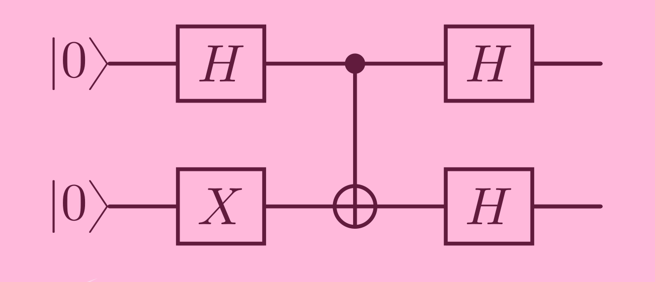
to summarise what we are looking at, this is a quantum circuit depicting two qubits with 3 stages to think about. i have split them up into "iteration 1", "iteration 2", "iteration 3" so you can follow each individual step. i don't know why i chose the word "iteration" anymore, but it made sense at the time and the image is annotated now so there's nothing i can do anymore. see the annotated version of this question below.

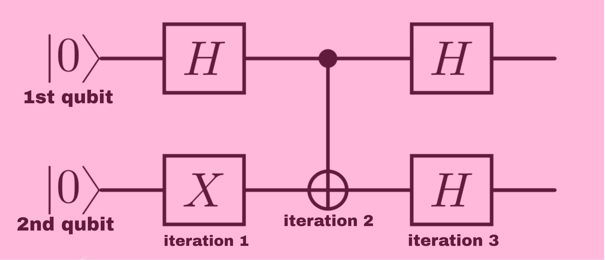
For iteration 1, we see that H is applied to the 1st qubit and X is applied to the 2nd. H is the Hadamard gate given by \( |H\rangle = \frac{1}{\sqrt{2}} \begin{pmatrix} 1 & 1 \\ 1 & -1 \end{pmatrix}\) and X is the unitary matrix given by \( X = \begin{pmatrix} 0 & 1 \\ 1 & 0 \end{pmatrix} \). Now we can apply each operation to the 1st and 2nd qubit respectively, both of which are currently in the state \( |0\rangle \ = \begin{pmatrix} 1 \\ 0 \end{pmatrix}\).

\[ H|0\rangle = |H\rangle = \frac{1}{\sqrt{2}} \begin{pmatrix} 1 & 1 \\ 1 & -1 \end{pmatrix} * \begin{pmatrix} 1 \\ 0 \end{pmatrix} = \frac{1}{\sqrt{2}}(|0\rangle + |1\rangle)\] \[X|0\rangle = \begin{pmatrix} 0 & 1 \\ 1 & 0 \end{pmatrix} * \begin{pmatrix} 1 \\ 0 \end{pmatrix} = |1\rangle \]

Now what is iteration 1 actually asking us to do? It's asking us to compute \(|\psi_{1}\rangle = H_{1} \otimes X_{2}\) where the subscripts denote which qubit (i.e the 1st or the 2nd) is being acted upon. We have computed these single qubit states already, so to do "iteration 1" we need to combine the results via the tensor product.

Iteration 1

\[|\psi_{1}\rangle = H_{1} \otimes X_{2} = \frac{1}{\sqrt{2}}(|0\rangle + |1\rangle) \otimes (|1\rangle)\] \[ = \frac{1}{\sqrt{2}}(|01\rangle + |11\rangle\]

Iteration 2

Iteration 2 is \(CNOT_{1->2}\), where the 1st qubit, x, is the control and the 2nd qubit, y, is the target. Recall that CNOT is given by \(|x,y\rangle = |x, x + y\rangle\)

\(0 + 1 = 1, 1 + 1 = 0,\) therefore applying CNOT to \(\frac{1}{\sqrt{2}}(|01\rangle + |11\rangle)\) gives us

\[ \frac{1}{\sqrt{2}}(|01\rangle + |10\rangle)\]

Iteration 3

Finally, we see that the final step is to apply H to both qubits. I hope you have been flicking back to the diagram and following so far. This is similar to iteration 1 in that we will operate on the single qubit states independently and then find the tensor product of them. We previously worked out that \( H|0\rangle = \frac{1}{\sqrt{2}}(|0\rangle + |1\rangle)\) and if you recall that \(|1\rangle = \begin{pmatrix} 0 \\ 1 \end{pmatrix}\) then we can deduce that \( H|1\rangle = \frac{1}{\sqrt{2}}(|0\rangle - |1\rangle)\)

This step isn't much more difficult than the previous ones, it's just longer because we have to take everything we have learned and apply this final operation to 4 qubits.

\[ (H \otimes I)\left[\frac{1}{\sqrt{2}}(|01\rangle + |10\rangle)\right] = \frac{1}{\sqrt{2}}\left[(H \otimes I)|01\rangle + (H \otimes I)|10\rangle\right] \] \[ = \frac{1}{\sqrt{2}}\left[(H|0\rangle)\otimes|1\rangle + (H|1\rangle)\otimes|0\rangle\right] \] \[ \frac{1}{\sqrt{2}}[\frac{1}{\sqrt{2}}\frac{1}{\sqrt{2}}(|0\rangle + |1\rangle)(|0\rangle - |1\rangle) + \frac{1}{\sqrt{2}}\frac{1}{\sqrt{2}}(|0\rangle - |1\rangle)(|0\rangle + |1\rangle)] \]

By expansion, we get:

\[ \frac{1}{\sqrt{2}}[\frac{1}{2}(|00\rangle - |01\rangle + |10\rangle - |11\rangle) + \frac{1}{2}(|00\rangle + |01\rangle - |10\rangle - |11\rangle)] \]

which simplifies to:

\[ \frac{1}{\sqrt{2}}(|00\rangle - |11\rangle)\]